
1. 임베딩(* Embedding)
워드 임베딩은 단어를 컴퓨터가 이해하고, 효율적으로 처리할 수 있도록 단어를 벡터화하는 기술입니다.
워드 임베딩은 단어의 의미를 잘 표현해야만 하며, 현재까지도 많은 표현 방법이 연구되고 있는 분야입니다.
워드 임베딩을 거쳐 잘 표현된 단어 벡터들은 벡터 공간에서 계산이 가능하며, 모델 투입도 가능합니다.
2. 인코딩(* Encoding)
기계는 자연어(* 영어, 한국어)를 이해할 수 없기 때문에, 데이터를 기계가 이해할 수 있도록 숫자 등으로 변환해주는 작업이 필수적입니다.
이런 작업을 인코딩(* Encoding)이라고 합니다.
텍스트 처리에서는 주로 정수 인코딩, 원 핫 인코딩을 사용합니다.
2.1 정수 인코딩
dictionary를 이용해서 정수 인코딩을 할 수 있습니다.
이는 각 단어와 정수 인덱스를 연결하고, 토큰을 변환해주는 인코딩 방식입니다.
text = '평생 살 것처럼 꿈을 꾸어라. 그리고 내일 죽을 것처럼 오늘을 살아라.'

tokens = [x for x in text.split(' ')]
unique = set(tokens)
unique = list(unique)

token2idx = {}
for i in range(len(unique)):
  token2idx[unique[i]] = i

encode = [token2idx[x] for x in tokens]
encode

# output:
# [5, 8, 9, 3, 2, 6, 7, 4, 9, 0, 1]
keras 를 통해서도 정수 인코딩을 할 수 있습니다.
dictionary, nltk 패키지를 이용한 방법들도 있지만, keras 에서는 텍스트 처리에 필요한 도구들을 지원합니다.
해당 도구는 자동으로 단어 빈도가 높은 단어의 인덱스는 낮게끔 설정합니다.
from tensorflow.keras.preprocessing.text import Tokenizer

text = '평생 살 것처럼 꿈을 꾸어라. 그리고 내일 죽을 것처럼 오늘을 살아라.'

t = Tokenizer()
t.fit_on_texts([text]) # 말뭉치가 입력이기 때문에, 리스트로 묶어서 입력해준다.
print(t.word_index)

encoded = t.texts_to_sequences([text])[0] # 마찬가지로 말뭉치가 출력이기에, 첫번째 인덱스만 출력한다.
print(encoded)

# output:
# {'것처럼': 1, '평생': 2, '살': 3, '꿈을': 4, '꾸어라': 5, '그리고': 6, '내일': 7, '죽을': 8, '오늘을': 9, '살아라': 10}
# [2, 3, 1, 4, 5, 6, 7, 8, 1, 9, 10]
2.2 원-핫 인코딩(* One-Hot Encoding)
원-핫 인코딩은 정수 인코딩한 결과를 벡터로 변환하는 인코딩 방식입니다.
원-핫 인코딩은 전체 단어 개수 만큼의 길이를 가진 배열에,
해당 정수를 가진 위치는 1, 나머지는 0을 가지는 벡터로 변환합니다.
이는 조건문을 통해 구현할 수도 있습니다.
import numpy as np

one_hot = []
for i in range(len(encoded)):
  temp = []
  for j in range(max(encoded)):
    if j == (encoded[i] - 1): # 같은 위치일때 1을 ..
      temp.append(1)
    else:
      temp.append(0)
  one_hot.append(temp)

np.array(one_hot)

# output:
'''
array([[0, 1, 0, 0, 0, 0, 0, 0, 0, 0],
       [0, 0, 1, 0, 0, 0, 0, 0, 0, 0],
       [1, 0, 0, 0, 0, 0, 0, 0, 0, 0],
       [0, 0, 0, 1, 0, 0, 0, 0, 0, 0],
       [0, 0, 0, 0, 1, 0, 0, 0, 0, 0],
       [0, 0, 0, 0, 0, 1, 0, 0, 0, 0],
       [0, 0, 0, 0, 0, 0, 1, 0, 0, 0],
       [0, 0, 0, 0, 0, 0, 0, 1, 0, 0],
       [1, 0, 0, 0, 0, 0, 0, 0, 0, 0],
       [0, 0, 0, 0, 0, 0, 0, 0, 1, 0],
       [0, 0, 0, 0, 0, 0, 0, 0, 0, 1]])
'''
원-핫 인코딩 또한 keras 를 통해 구현할 수도 있습니다.
from tensorflow.keras.utils import to_categorical

one_hot = to_categorical(encoded)
one_hot

# output:
'''
array([[0., 0., 1., 0., 0., 0., 0., 0., 0., 0., 0.],
       [0., 0., 0., 1., 0., 0., 0., 0., 0., 0., 0.],
       [0., 1., 0., 0., 0., 0., 0., 0., 0., 0., 0.],
       [0., 0., 0., 0., 1., 0., 0., 0., 0., 0., 0.],
       [0., 0., 0., 0., 0., 1., 0., 0., 0., 0., 0.],
       [0., 0., 0., 0., 0., 0., 1., 0., 0., 0., 0.],
       [0., 0., 0., 0., 0., 0., 0., 1., 0., 0., 0.],
       [0., 0., 0., 0., 0., 0., 0., 0., 1., 0., 0.],
       [0., 1., 0., 0., 0., 0., 0., 0., 0., 0., 0.],
       [0., 0., 0., 0., 0., 0., 0., 0., 0., 1., 0.],
       [0., 0., 0., 0., 0., 0., 0., 0., 0., 0., 1.]])
'''
3. 데이터 수집 및 전처리
인터넷 영화 데이터베이스인 IMDb 의 5만개의 리뷰 데이터셋을 이용합니다.
우선 사용할 모듈들을 import 합니다.
from tensorflow.keras.datasets import imdb
from tensorflow.keras.models import Sequential
from tensorflow.keras.layers import Embedding, Dense, Flatten
단어의 개수를 1000개로 설정한 후,
데이터를 받아옵니다.
정답 레이블은 긍정과 부정을 뜻하는 1과 0으로 이루어진 벡터입니다.
num_words = 1000 # 단어 개수 설정

(X_train, y_train), (X_test, y_test) = imdb.load_data(num_words=num_words)

print(X_train.shape)
print(y_train.shape)
print(X_test.shape)
print(y_test.shape)

# output:
# (25000,)
# (25000,)
# (25000,)
# (25000,)

# 단어 인코딩 값과 정답 레이블 출력
for i in range(10):
  if y_train[i] == 0:
    label = '부정'
  else:
    label = '긍정'

  print(f'{X_train[i]}\n{label}')

# output:
'''
[1, 14, 22, 16, 43, 530, 973, 2, 2, 65, 458, 2, 66, 2, 4, 173, 36, 256, 5, ...]
긍정
[1, 194, 2, 194, 2, 78, 228, 5, 6, 2, 2, 2, 134, 26, 4, 715, 8, 118, 2, 14, ...]
부정
[1, 14, 47, 8, 30, 31, 7, 4, 249, 108, 7, 4, 2, 54, 61, 369, 13, 71, 149, 14, ...]
부정
[1, 4, 2, 2, 33, 2, 4, 2, 432, 111, 153, 103, 4, 2, 13, 70, 131, 67, 11, 61, ...]
긍정
[1, 249, 2, 7, 61, 113, 10, 10, 13, 2, 14, 20, 56, 33, 2, 18, 457, 88, 13, 2, ...]
부정
[1, 778, 128, 74, 12, 630, 163, 15, 4, 2, 2, 2, 2, 32, 85, 156, 45, 40, 148, ...]
부정
[1, 2, 365, 2, 5, 2, 354, 11, 14, 2, 2, 7, 2, 2, 2, 356, 44, 4, 2, 500, 746, 5, ...]
긍정
[1, 4, 2, 716, 4, 65, 7, 4, 689, 2, 2, 2, 2, 2, 2, 2, 2, 2, 2, 2, 2, 2, 4, 2, ...]
부정
[1, 43, 188, 46, 5, 566, 264, 51, 6, 530, 664, 14, 9, 2, 81, 25, 2, 46, 7, 6, ...]
긍정
[1, 14, 20, 47, 111, 439, 2, 19, 12, 15, 166, 12, 216, 125, 40, 6, 364, 352, ...]
부정
'''
데이터를 받은 후,
데이터 전처리를 해줍니다.
모든 데이터의 길이를 같게 만들어줘야 합니다.
이를 pad_sequence() 메소드를 통해 구현합니다.
데이터의 길이가 maxlen 보다 길면 데이터를 자르고,
데이터의 길이가 maxlen 보다 짧으면 padding 설정에 따른 값을 추가해줍니다.
(* pre: 데이터의 앞을 0으로 채움, post: 데이터의 뒤를 0으로 채움)
모든 데이터(* 문장 하나하나)가 같은 길이로 맞아야 Embedding 레이어를 사용할 수 있습니다.
from tensorflow.keras.preprocessing.sequence import pad_sequences

max_len = 100

pad_x_train = pad_sequences(X_train, maxlen=max_len, padding='pre')
pad_x_test = pad_sequences(X_test, maxlen=max_len, padding='pre')

print(len(X_train[0])) # before padding
print(len(pad_x_train[0])) # after padding

# output:
# 218
# 100
4. 모델 구성
keras 를 이용해 아키텍쳐를 구현합니다.
Embedding Layer 와 이후 처리의 간편함을 위해 Flatten() 을 넣어주고,
sigmoid 를 활성화 함수로 갖는(* 이진 분류, 긍정/부정) Layer 를 추가해줍니다.
model = Sequential()

model.add(Embedding(input_dim=num_words, output_dim=32))
model.add(Flatten())
model.add(Dense(1, activation='sigmoid'))

model.compile(optimizer='rmsprop',
              loss='binary_crossentropy',
              metrics=['acc'])

history = model.fit(pad_x_train, y_train,
                    epochs=10, batch_size=32,
                    validation_split=0.2)
그 후 결과를 시각화 해줍니다.
import matplotlib.pyplot as plt
plt.style.use('seaborn-white')

hist_dict = history.history
print(hist_dict.keys())

# output:
# dict_keys(['acc', 'loss', 'val_acc', 'val_loss'])

plt.plot(hist_dict['loss'], 'b-', label='Train Loss')
plt.plot(hist_dict['val_loss'], 'r:', label='Validation Loss')
plt.legend()
plt.grid()

plt.figure()
plt.plot(hist_dict['acc'], 'b-', label='Train Accuracy')
plt.plot(hist_dict['val_acc'], 'r:', label='Validation Loss')
plt.legend()
plt.grid()

plt.show()
결과
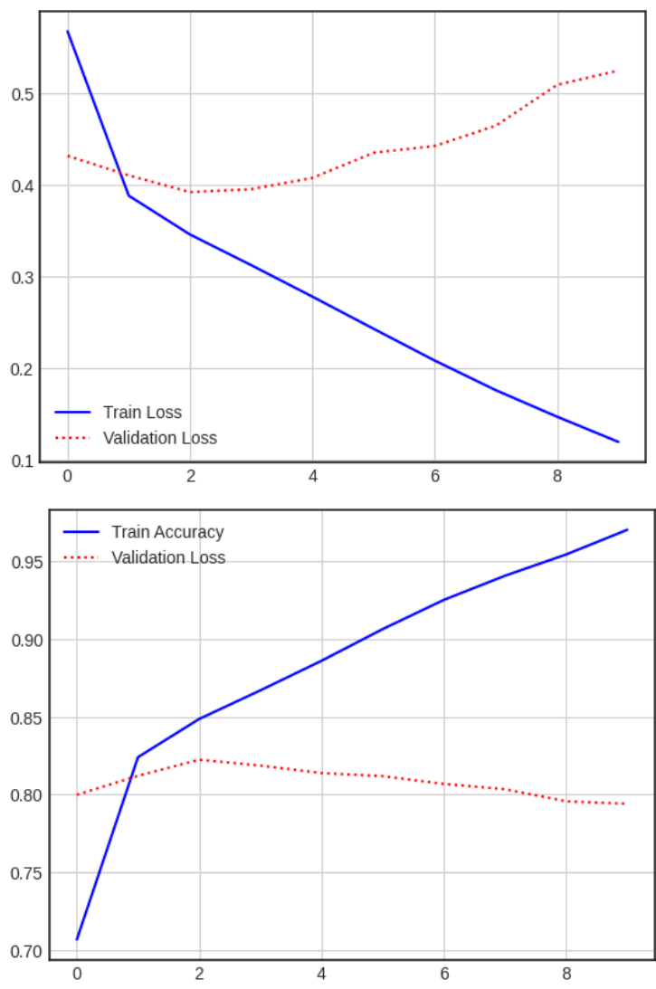
평가
모델이 오버피팅이 된 모습을 볼 수 있습니다.
단어의 수를 늘린 후 재학습해보겠습니다.
num_words=2000
max_len=400

(X_train, y_train), (X_test, y_test) = imdb.load_data(num_words=num_words)

pad_x_train_2 = pad_sequences(X_train, maxlen=max_len, padding='pre')
pad_x_test_2 = pad_sequences(X_test, maxlen=max_len, padding='pre')

model = Sequential()

model.add(Embedding(input_dim=num_words, output_dim=32))
model.add(Flatten())
model.add(Dense(1, activation='sigmoid'))

model.compile(optimizer='rmsprop',
              loss='binary_crossentropy',
              metrics=['acc'])

history_2 = model.fit(pad_x_train_2, y_train,
                    epochs=10, batch_size=32,
                    validation_split=0.2)
시각화를 해줍니다.
import matplotlib.pyplot as plt
plt.style.use('seaborn-white')

hist_dict = history_2.history
# print(hist_dict.keys())

plt.plot(hist_dict['loss'], 'b-', label='Train Loss')
plt.plot(hist_dict['val_loss'], 'r:', label='Validation Loss')
plt.legend()
plt.grid()

plt.figure()
plt.plot(hist_dict['acc'], 'b-', label='Train Accuracy')
plt.plot(hist_dict['val_acc'], 'r:', label='Validation Loss')
plt.legend()
plt.grid()

plt.show()
결과
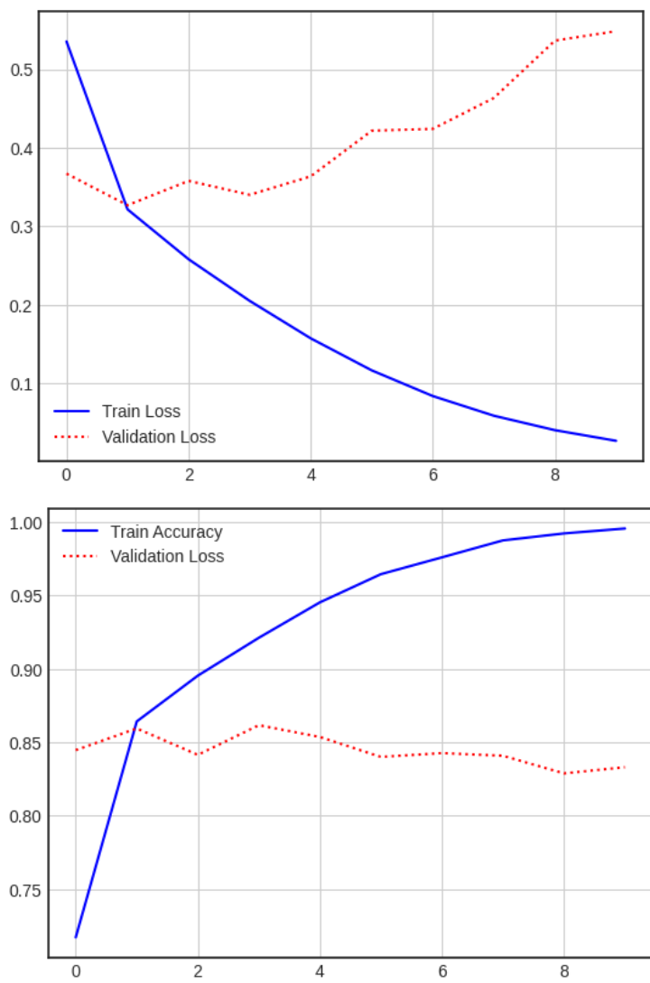
이 전보다 정확도가 많이 좋아졌지만, 오버피팅 문제는 해결되지 않았습니다.
이는 해당 모델이 단어간의 관계나 문장 구조 등 의미적 연결을 전혀 고려하지 않기 때문입니다.
이를 해결하기 위해서는,
시퀀스 전체를 고려한 특성을 학습시킬 수 있는 RNN 층이나 1D CNN 층을 Embedding 층 위에 추가해야 합니다.
5. Word2Vec
2024.08.16 - [[Deep daiv.] 복습] - [Deep daiv.] TIL - 6. Word2Vec을 활용한 단어 임베딩
[Deep daiv.] TIL - 6. Word2Vec을 활용한 단어 임베딩
0. 현재 상황 2024.08.14 - [[Deep daiv.] 복습] - [Deep daiv.] TIL & WIL - 5. 자연어 처리 & 텍스트 처리 (Contd.) [Deep daiv.] TIL & WIL - 5. 자연어 처리 & 텍스트 처리 (Contd.)이전 글2024.08.09 - [[Deep daiv.] NLP] - [Deep daiv.
hw-hk.tistory.com
6. t-SNE
2024.08.09 - [[Deep daiv.] 복습] - [Deep daiv.] TIL - 3.1 차원축소와 클러스터링
[Deep daiv.] TIL - 3.1 차원축소와 클러스터링
1. PCA 주성분 분석 고차원의 데이터를 낮은 차원의 데이터로 바꿀 때, 어떻게 바꿔야 최대한 특징을 살리면서 차원을 낮출 수 있을까를 고안하다가 나온것이 PCA 입니다. 그렇다면 어떻게 해야 '
hw-hk.tistory.com
Word2Vec 을 통해 임베딩한 단어들을 차원축소를 통해 시각화 할 수 있습니다.
배움
keras를 통한 감성 분석 예제
'[Deep daiv.] > [Deep daiv.] NLP' 카테고리의 다른 글
| [Deep daiv.] NLP, WIL - 7.1 Seq2seq 실습 (1) | 2024.09.06 |
|---|---|
| [Deep daiv.] WIL, NLP - 8. 순환 신경망 실습 (6) | 2024.09.02 |
| [Deep daiv.] WIL, NLP - 7. Seq2seq with Attention (0) | 2024.08.29 |
| [Deep daiv.] WIL, NLP - 5. 토픽 모델링 (0) | 2024.08.22 |
| [Deep daiv.] WIL, NLP - 4. 의미 연결망 분석(Sematic Network Analysis) (0) | 2024.08.21 |