[Computer Architecture] Instructions: Language of the Computer part 2 | Week 5

Six Steps in Procedure Calling

 

함수를 호출하는 경우 다음의 6가지 과정을 거칩니다:

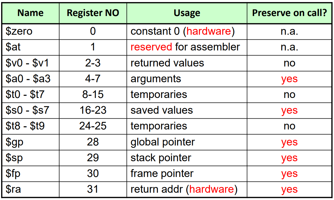
1. Main routine (caller) places parameters in a place where the procedure (callee) can access them; caller는 callee가 사용할 수 있는 공간에 파라미터들을 옮깁니다. *$a0 - $a3: four argument registers
2. Caller transfers control to the callee; caller는 callee에게 통제권을 넘깁니다. *이 경우 callee가 caller의 register정보들을 memory(stack)에 저장해줍니다.
3. Callee acquires the storage resources needed; callee는 필요한 자원을 register에 load합니다.
4. Callee performs the desired operations; callee는 원하는 연산을 수행합니다.
5. Callee places the result value in a place where the caller can access it; callee는 caller가 사용할 수 있는 공간에 return value를 옮깁니다. *$v0 - $v1: two value registers for result values
6. Caller returns control to the caller; callee는 caller에게 통제권을 넘깁니다. *$ra: one return address register to return to the point of origin

Register Usage

 

Instructions for Procedure Call

 

MIPS에서는 procedure call을 다음의 명령을 통해 수행합니다:

jal ProcedureAddress # jump and link

 

이는 현재 PC+4 의 값을 $ra에 저장한 후, procedure address에 해당하는 곳으로 이동하는 명령입니다. 이는 target address로 바로 이동하기 때문에 J-format 명령을 사용합니다.

 

그리고 procedure return을 하고싶은 경우 다음의 명령을 사용합니다:

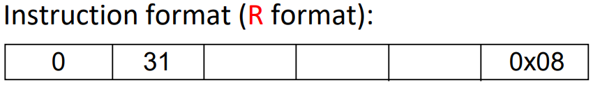
jr $ra #return

 

이는 $ra에 있는 값을 PC로 옮기는 기능을 수행합니다. 이는 R-format을 사용합니다.

jr

 

Leaf Procedure Example

 

int leaf_example(int g, h, i, j)
{
    int f;
    f = (g + h) - (i + j);
    return f;
}

 

위와 같은 C code가 있는 경우 다음과 같이 표현됩니다:

# Arguments g, ..., j in $a0, ..., $a3
# f in $s0 (hence, need to save $s0 on stack)
# Result in $v0

leaf_example:
             addi $sp, $sp, -12
             sw $t1, 8($sp)          # save $t1 on stack
             sw $t0, 4($sp)          # save $t0 on stack
             sw $s0, 0($sp)          # save $s0 on stack
             
             # procedure body
             add $t0, $a0, $a1
             add $t1, $a2, $a3
             sub $s0, $t0, $t1
             
             # result
             add $v0, $s0, $zero
             
             lw $s0, 0($sp)          # restore $s0
             lw $t0, 4($sp)          # restore $t0
             lw $t1, 8($sp)          # restore $t1
             addi $sp, $sp, 12
             
             # return
             jr $ra

 

Non-Leaf Procedures

 

procedure안에서 다른 procedure를 부르는 경우를 말합니다. 이는 caller는 자기 자신을 호출한 caller에 대한 정보들을 stack에 미리 저장해놔야합니다. 그래서 caller는 $ra와 $a0, ... 들을 저장해야합니다. *자신이 caller에게 돌아가기 위함 + caller로부터 받은 데이터들을 저장하기 위해, callee가 덮어써버릴 것이기 때문에...

 

Non-Leaf Procedure Example

 

int fact(int n)
{
    if (n<1) return 1;
    else return n * fact(n-1);
}

 

위 함수의 경우 caller가 callee가 될 수 있기 때문에, caller가 자신의 정보를 미리 stack에 저장해야합니다. 이를 어셈블리 코드로 나타내면 다음과 같습니다:

# Argument n in $a0
# result in $v0

fact:
     addi $sp, $sp, -12     # adjust stack for 3 items
     sw $ra, 8($sp)        # save return address
     sw $a0, 4($sp)        # save argument
     sw $t0, 0($sp)        # save temporary
     
     # test for n < 1
     slti $t0, $a0, 1
     beq $t0, $zero, L1
     
     # if so, result is 1, pop 3 items from stack and return
     addi $v0, $zero, 1
     addi $sp, $sp, 12
     jr $ra
     
L1:  
     addi $a0, $a0, -1     # else decrement n
     jal fact              # recursive call
     
     # restore original n and return address
     lw $a0, 4($sp)
     lw $ra, 8($sp)
     addi $sp, $sp, 12     # pop 3 items from stack
     
     mul $v0, $a0, $v0     # multiply to get result
     jr $ra                # and return

 

Aside: Spilling Registers

 

Callee가 return value와 argument들을 사용할 때 register의 개수를 초과한다면 이를 spilling register라고 부르며, stack에 값을 저장합니다.

Spilling register

 

함수 호출시 stack의 변화는 다음과 같습니다:

Local Data on the Stack

 

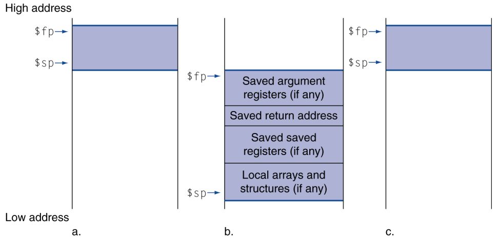
*이때 $fp는 함수의 시작을 나태내는, procedure의 시작을 나타내는 frame pointer입니다. 이때의 procedure frame을 activation record라고 부릅니다.

 

Aside: allocation space on the heap

 

procedure가 실행되는 경우 memory공간은 다음과 같습니다:

Allocating Space on the Heap

 

이때 static data segment는 global이나 static으로 선언된 데이터들이 저장되어있으며, 이들은 $gp에 의해 pointing됩니다. Stack의 경우는 함수에서 사용되는 local 변수들이나, return address들이 저장되는 공간이며 위에서 아래로 길어지는 형태를 갖습니다. heap의 경우는 linked list와 같이 실행시간에 능동적으로 생기는 데이터들이 저장되는 공간입니다. 이는 C에서 malloc()을 통해 데이터를 생성할 수 있으며, free()를 통해 deallocation을 할 수 있습니다. *예를 들어 A[100]과 같이 배열을 선언하면 Stack에, malloc(A*100)과 같이 선언하면 heap에 데이터가 생성됩니다.

 

Addressing Model Summary

 

Addressing Mode Summary

 

MIPS에서 봤던 addressing 타입은 다음과 같습니다.

 

Synchronization

 

동기화는 race condition을 막기 위해 필수적입니다. race condition은 두 개 이상의 서로 다른 쓰레드가 하나의 공간에 위치한 데이터에 접근하는 경우에 발생할 수 있습니다.

2024.09.28 - [[학교 수업]/[학교 수업] System Programming] - [시스템 프로그래밍] Race Condition

[시스템 프로그래밍] Race Condition

 

이런 동기화는 HW의 지원이 필요합니다. 예를 들어 원자성을 보장받는 read/write memory 명령등이 있습니다.

 

Atomic Exchange Support

 

Atomic exchange (atomic swap)은 memory에 있는 값을 register로 옮길 때 하나의 operation과 같이 수행할 수 있도록 도와줍니다. 이는 다음의 명령들을 통해 구현됩니다:

• Load linked: ll rt, offset(rs)
• Store conditional: sc rt, offset(rs)
  • sc명령은 지정한 메모리 공간의 값이 ll명령이 있고난 후 변화가 있다면 0을, 변화가 없다면 1을 rt에 저장합니다. 이를 통해 ll연산 후 계산을 수행하는 동안의 원자성을 보장할 수 있습니다.

 

Atomic Exchange with ll and sc

 

try: 
    add $t0, $zero, $s4    # $t0=$s4 (exchange value)
    ll $t1, 0($s1)         # load memory value to $t1
    sc $t0, 0($s1)         # try to store exchange value to memory, if fail $t0 will be 0
    
    beq $t0, $zero, try    # try again if store fails
    add $s4, $zero, $t1    # load value in $s4

 

이는 ll과 sc사이에서 메모리 값의 변화가 있다면, 이를 다시 수행하는 코드입니다.

 

Assembler Pseudoinstructions

 

대부분의 어셈블러 명령은 기계어 명령과 one-to-one 관계를 갖습니다. 하지만 어셈블러에 의해 변경된 명령들을 Pseudoinstructions라고 부릅니다.

• move $t0, %t1 → add $t0, $zero, $t1
• blt $t0, $t1, L → slt $at, $t0, $t1 / bne $at, $zero, L

 

Translation and Startup

 

Translation and Startup

 

Linking Object Modules

 

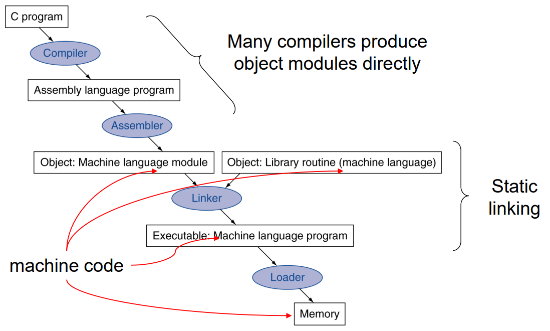
obj파일들을 하나의 실행가능한 이미지로 만드는 작업을 linking이라고 합니다. 이는 다음의 단계를 따릅니다:

1. Merges segments; segment들을 병합합니다.
2. Resolve labels (determine their addresses); 각각의 (procedure호출때 사용할 procedure의) 주소들을 레이블링 해줍니다.
3. Patch location-dependent and external refs; 외부 레퍼런스를 통해 absolute location을 계산합니다.

사실 linking과정에서 procedure들의 주소를 레이블링하는 경우 virtual memory를 사용한다면 상대 주소만 알면 되기 때문에 absolute location을 구할 필요는 없습니다. program이 실행될 때 이를 계산하면 됩니다.

 

Loading a Program

 

프로그램이 memory로 load되어 실행되는 과정은 다음과 같습니다:

1. Read header to determine segment sizes; 헤더를 읽어 segment의 크기를 결정합니다.
2. Create virtual address space; 이에 해당하는 가상 메모리 공간을 생성합니다.
3. Copy text and initialized data into memory; 코드 text를 복사하고, 시작 데이터를 메모리에 load합니다.
4. Set up arguments on stack; 파라미터들을 stack에 세팅합니다.
5. Initialize registers (including $sp, $fp, $gp); 프로그램 실행에 사용되는 레지스터들을 초기화해줍니다.
6. Jump to startup routine; 시작합니다.

 

Compiler Benefits

 

좋은 compiler는 좋은 성능을 만들어줍니다. 아래는 bubble 정렬을 할 때 compiler별로의 성능 비교입니다:

To sort 100,000 words with the array initialized to random values on a Pentium 4 with a 3.06 clock rate, a 533 MHz system bus, with 2 GB of DDR SDRAM, using Linux version 2.4.20

 

Clock cycle의 측면에서는 O3가, Instr count의 측면에서는 O1이, CPI의 측면에서는 None이 좋습니다. 즉, 다시한번 Instr count나 CPI는 절대적인 성능과 관련이 없습니다.

 

ARM & MIPS Similarities

 

ARM은 가장 유명한 embedded core로 RISC의 대표주자입니다.

ARM $ MIPS Similarities

 

다음에 나오는 그림들은 MIPS와 ARM의 차이점과 공통점들 입니다.

Compare and Branch in ARM

Instruction Encoding

 

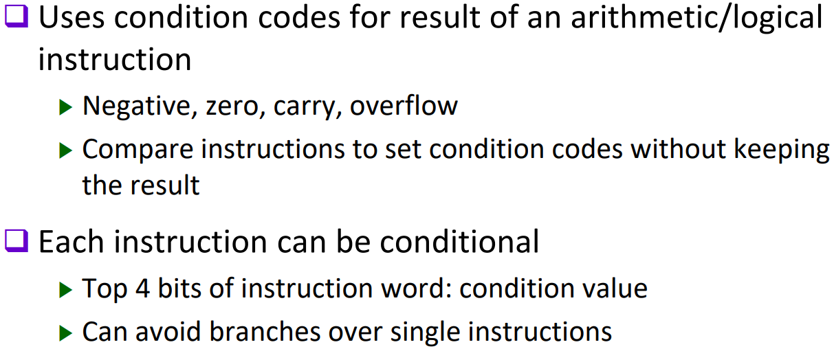
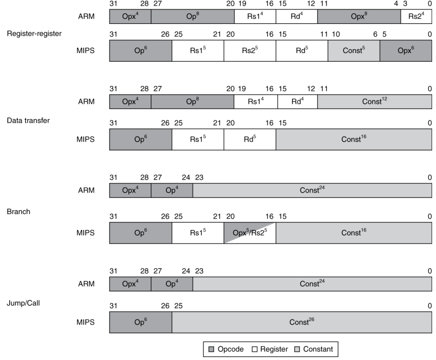
*MIPS와 유사하게 고정된 길이의 instruction encoding을 사용합니다.

 

ARM v8 Instruction의 특징

 

The Intel x86 ISA

 

x86은 CISC의 대표주자입니다.

Basic x86 Registers

 

Basic x86 Addressing Models

 

*MIPS와 달리 2개의 operand밖에 없지만 (MIPS는 최대 3개, source 2개 destination 1개), 사용가능한 source의 종류가 더 많습니다 (MIPS와 달리 memory operand도 사용 가능합니다).

 

 

x86 Instruction Encoding

 

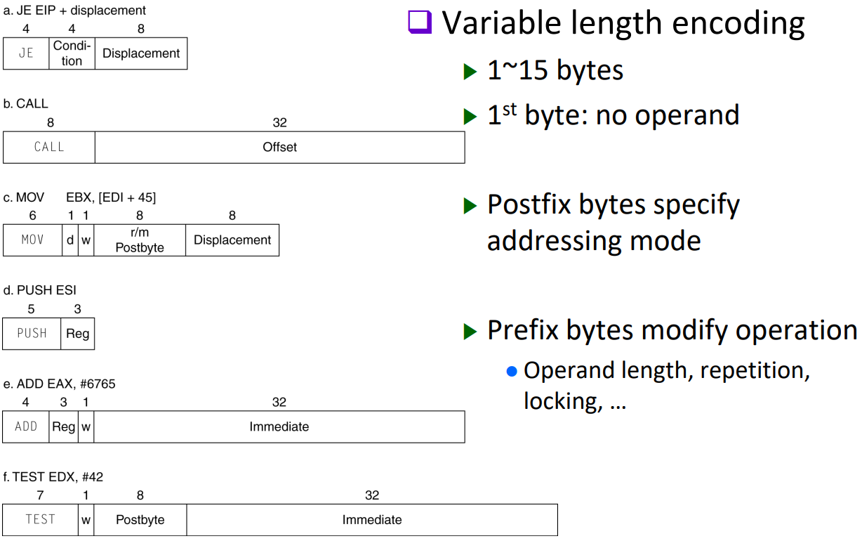
*MIPS와 달리 고정 길이 instruction encoding이 아닙니다.

 

 

Implementing IA-32

 

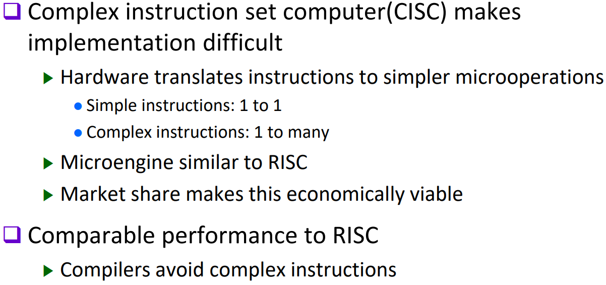
CISC는 고정 길이 instruction encoding이 아니기 때문에 구현이 매우 어렵습니다. 그렇기 때문에 그 중간에 microengine을 통해 CISC instruction을 RISC likely하게 변경한 후 RISC와 비슷한 microoperation들로 잘게 쪼개서 명령을 수행합니다. 즉, 이는 RISC와 유사하게 구현됨을 알 수 있습니다.

 

Fallacies

 

• Powerful instruction → higher performance?
  
  • CISC는 성능이 좋지 않습니다..
• Write assembly code to obtain the high performance?
  • 현대의 compiler는 너무 정교해서 인간에 비해 성능 향상의 비율이 더 좋습니다.
  • 또한 해석력이 부족하기 때문에 error나 생산성의 측면에서 비효율입니다.
• Backward Compatibility → instruction set doesn't change?
  • 이전 버전의 instruction들을 지원해주면서 새로운 instruction들을 개발하기 때문에 # instruction은 계속 늘어나고 있습니다.

# of x86 instruction set

 

Pitfalls

 

• Sequential word는 연속된 메모리 공간에 할당되지 않습니다!
  
  • word는 4byte단위이고, memory 주소는 byte단위이기 때문입니다.